Article Text

Statistics from Altmetric.com
Healthcare professionals and policy makers are increasingly aware of the need for their decisions to be informed by the best available research evidence. Although the articles selected for abstraction in Evidence-Based Nursing have already been appraised, and only the highest quality research selected, practitioners still need basic skills to identify and interpret methodologically sound research. This editorial is one of a series that aims to help you to do this, and is the second of 3 editorials focusing on some basic measurement and statistical issues in healthcare research. In this editorial, we look at how the results of intervention or “treatment” studies are summarised and presented for different types of health outcomes. The next editorial will explain how statistical techniques are used to assess the probability that the observed treatment effect occurred by chance, and what is meant by a “statistically significant” result.EBN notebook
Measures of health and disease
Many measures are used to assess the health outcomes of an intervention, ranging from those trying to capture its effect on people's general health (eg, Short Form-36) to measures of a specific dimension relevant to a particular disease (eg, the Beck Depression Inventory). Some are measures of patients' perceptions of their health; more often, however, they are measures that clinicians or researchers think are important. Regardless, these measures are generally either continuous or discrete; this distinction is important because the type of measure used determines the way the results are presented and analysed.
CONTINUOUS MEASURES
When the outcomes of a study are continuous (eg, temperature, blood pressure, or cholesterol concentrations), the researchers are usually interested in the extent to which these values change after exposure to an intervention. Studies that use continuous outcome measures may compare the average values of the variable (eg, mean or median) after treatment. In a study of treatment for arthritis, researchers may measure changes in levels of pain or mobility on one or more pain or mobility scales. In conditions that are life threatening, studies may assess outcomes such as length of survival.
Recently, emphasis has shifted to more patient centred measures of health. These measures assess patient ratings of health along several dimensions, such as physical functioning, social functioning, mental health, and pain, and either score these separately in the form of a health profile (eg, Nottingham Health Profile) or combine the ratings of different dimensions into a single number or index (eg, Euroqol or General Health Questionnaire). All of these use continuous scales.
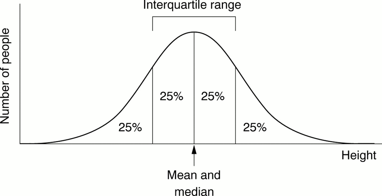
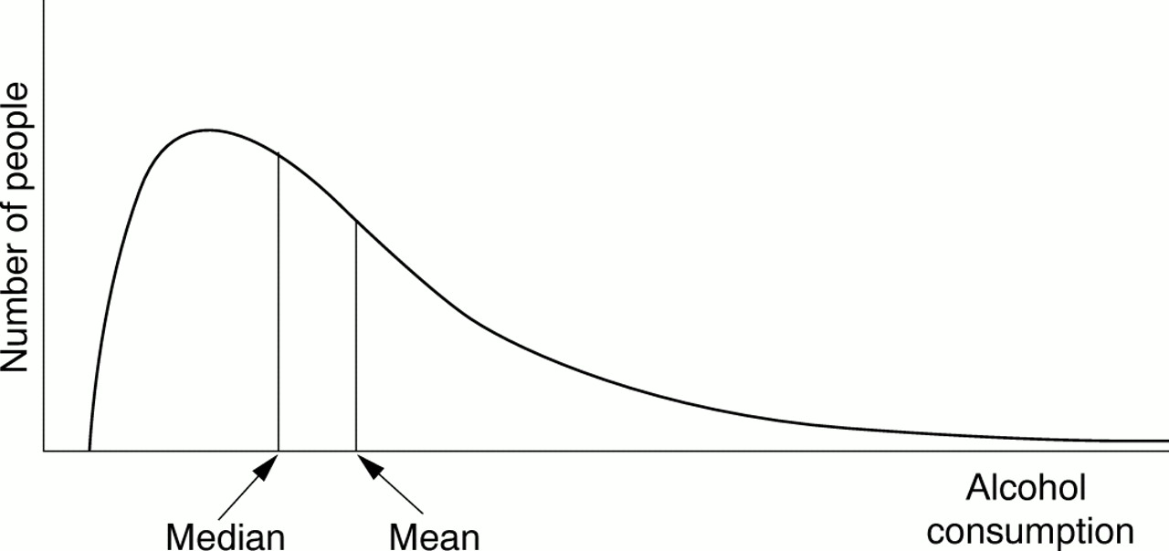
Once the change in score has been determined for each individual patient, the overall change in score for the group that received the intervention is compared with the overall change in score for the control group. How is this done? Many biological phenomena, such as height, are distributed “normally” in the population. The term normal in this context refers to the symmetrical bell shaped curve when the values for a large sample are plotted. Most values cluster around the middle value, with fewer at either end of the scale (fig 1⇓). The scores for a group of people are usually summarised by the use of an average—either the mean or the median. The mean is calculated by adding all the values together and dividing by the number of observations. The median is the value of the middle observation when all the observations are put in order; 50% of the observations lie above the median and 50% lie below. When data are normally distributed, the mean and median are equal and the mean value is used to summarise the data; however, when data are not normally distributed, also known as a “skewed distribution” (fig 2⇓), it is more informative to use the median rather than the mean value to summarise the data. Because not everyone in a group responds to an intervention in the same way or to the same degree, we also should know something about the extent to which the values are spread out or dispersed. This can be done by describing the range of values in a group (the minimum and maximum values recorded). Other methods of recording this dispersion include the interquartile range, between which 50% of all the observations lie, or the standard deviation (SD), which is a measure of the average amount individual values differ from the mean in that group; the lower the SD, the smaller the spread of values.

A normal distribution curve: variables such as height are distributed like this in the population.

A skewed distribution curve: variables such as alcohol consumption are distributed like this.
DISCRETE MEASURES
Instead of measuring health outcomes on a continuous scale, studies often focus on discrete health events, such as the occurrence of a disease, death, or hospital discharge. What these outcomes have in common is that the event either occurs or does not; they are discrete measures (often termed dichotomous).
For a group of people, discrete outcomes can be summarised as the percentage or proportion of people who experience an event during the follow up period. For example, in the study of pressure bandages after coronary angioplasty by Botti et al (see Evidence-Based Nursing, July 1999, p84), 3.5% of patients with a pressure bandage experienced bleeding compared with 6.7% of those without a bandage. These proportions express the probability or risk that a person in the group of interest experienced the event at some point during the follow up period.
This summary measure can be extended to take into account not only whether people experienced the event but also the rate at which they did so. For example, if 20% of the men in a study are dead after 2 years, the risk of men dying by 2 years would be 20% regardless of whether they all died by 1 year or 2 years. The rate, however, measures the number of people experiencing the event per unit of time (incidence). If all deaths occurred by 1 year, the rate would be 20 per 100 person years (20 deaths for each 100 people followed up for 1 year), whereas if they all died by 2 years, the incidence would be halved or 10 per 100 person years.
Continuous measures are often expressed as discrete ones in evaluative studies, especially if there is a threshold above or below which there is a clinical difference. For example, scales that measure depression can be used to measure the values of the depression score (ie, the extent of the depression) or to assign a value to the score above which a patient can receive a diagnosis of depression. In other words, the first approach measures how depressed people were before and after treatment, whereas the second uses a threshold measure to classify whether more or fewer people were depressed at the end of treatment compared with before the treatment. A good example of the second approach can be found in the review of St John's Wort by Linde and Mulrow (Evidence-Based Nursing, July 1999, p82) where patients were classed as “responders” or “non-responders” to treatment.
Measures of effect and association
The previous section described different ways of measuring health outcomes. In this section we will examine how these measures are used to determine whether an intervention has an effect on an outcome and the size and direction of this effect. As before, the approach depends on whether the outcome is measured as a continuous or discrete variable. Remember that differences in the outcomes of the patients who receive different interventions are not necessarily caused by the interventions. Association does not imply causation. It may be that the patients in the groups were different to begin with, or were managed differently in other respects, or that the outcomes were assessed differently. These are important criteria by which treatment studies should be appraised and will be the subject of future Notebook editorials. It could also be that differences occurred by chance; one of the purposes of statistical analysis is to determine whether this is likely to be the case.
CONTINUOUS MEASURES
Studies that use continuous outcome measures often compare the mean (or median) values of the outcome or the average change in outcome for the intervention and control groups. If the average values (or changes) differ, then it suggests that there are differences in the effect between the intervention and the control conditions. For example, in a trial of bereavement support for homosexual men (Evidence-Based Nursing, October 1999, p116), the researchers used a composite score for grief and distress and measured this before and after bereavement support in the treatment group, and before and after standard care in the control group. They then compared the mean change (in this case, a decrease) in the distress-grief composite score in each group and found a significantly greater reduction in the group that received bereavement support.
Another way of expressing differences in outcome for continuous measures is by dividing the difference in means by the SD. This is called the standardised difference and has no units. It simply expresses the effect of an intervention in terms of the number of SDs apart the averages of the 2 groups are. This allows comparison of the size of the treatment effect when different outcome measures are used and has therefore been used in meta-analyses, which attempt to compare and combine the results of several studies. You will often encounter reporting of standardised differences when reading systematic reviews in the Cochrane Library. Because standardised differences have no units, however, they have no direct clinical meaning and so are difficult to interpret.
DISCRETE MEASURES
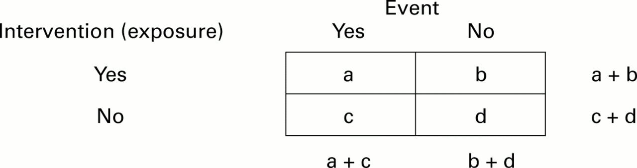
The measure of effect when using discrete outcomes (eg, dead or alive) compares the risk of an event in the intervention and control groups; figure 3⇓ illustrates this.
Numbers of people who receive (don't receive) an intervention and who have (don't have) an event.
The risk of an event in the intervention group is simply the proportion of people in that group who experience the event,

The corresponding risk in the control group is:

There are 2 ways in which the outcome, or event rates, can be compared in participants who receive and do not receive the intervention. The relative risk (RR) or risk ratio is the risk of patients in the intervention group experiencing the outcome divided by the risk of patients in the control group experiencing the outcome.

If the intervention and control conditions have the same effect, then (assuming the groups are comparable in all other respects) the risk of the event (eg, death) will be the same in both groups, and the RR will be 1.0. If the risk of death is reduced in the intervention group compared with the control group, then the RR will be <1.0. If, however, the intervention is harmful, then the RR will be >1.0. The further away the RR is from 1.0, the greater the strength of the association between the intervention and the outcome.
For various statistical reasons, some studies express the outcome as the odds of the event (a/b) rather than the risk of the event (a/a+b). The odds ratio (OR) is the odds of the event in the intervention group (a/b) divided by the odds of the event in the control group (c/d):

As with the RR, an OR of 1.0 means there is no difference between the groups and an OR <1.0 means that the event is less likely in the intervention group than the control group. Thus, in the trial of nurse led secondary prevention clinics (Evidence-Based Nursing, January 1999, p21), nurse led clinics significantly reduced the odds of hospital admission compared with usual care (OR=0.64); that is, there was a 36% (1.0-0.64) reduction in the odds of hospital admission. When the event being measured is quite rare, the OR and RR are numerically similar because the values of a and c are insignificantly small.
Clinical importance
ORs and RRs are measures of the strength of association between an intervention and an outcome. However, they do not tell us much about the impact or clinical significance of the intervention, and therefore whether the intervention is worth considering.
It is important to remember that the RR indicates the relative benefit of a treatment, not the actual benefit; that is, it does not take into account the number of people who would have developed the outcome anyway, which is captured by the absolute risk difference—known as absolute risk reduction (ARR) when risk is reduced. The ARR can be calculated by simply subtracting the proportion of people experiencing the outcome in the intervention group from the proportion experiencing the outcome in the control group. The absolute difference in risk tells us how much the reduction is a result of the intervention itself.
For example, in a study of depression, if 2% of participants in the control group are depressed (ie, Rc = 0.02) and a treatment halves the risk of depression to 1% (ie, Ri = 0.01), then the RR is:

A RR of 0.5 or a halving of the risk looks like a large effect, but the absolute difference in risk is only:

This is a risk reduction of only 1 event per 100 people. This sounds a lot less impressive than a statement that it halves the risk of depression. So, when reading a report of an intervention study, we need to interpret the RR or OR within the context of how frequently the outcome occurs in the population.
Another approach to expressing the effect of an intervention is the number needed to treat (NNT), which conveniently expresses the absolute effect of the intervention. This is simply 1 divided by the absolute risk difference:

In other words, one would need to treat 100 patients to prevent one additional case of depression. The NNT represents the number of patients who would need to be treated to prevent one additional event and is a useful way of expressing clinical effectiveness—the more effective an intervention, the lower the NNT.
To illustrate this, consider the impact of the same intervention, which still halves the risk of depression in the treatment group compared with the control group, but this time, in a population at higher risk. If the risk of the event in the control group (Rc) is now 0.2 (ie, 20% experience the event), then the risk in the intervention group (Ri) will be 0.1 (ie, 10% experience the event). Now the absolute risk difference is 0.2–0.1=0.1, and the NNT is 1/0.1=10. In other words, only 10 people would need to be treated to prevent one additional case of depression. The effectiveness of the treatment in terms of the OR or RR is the same, but the impact is much greater because the risk of depression in the untreated group is so much higher.
A recent example of how the difference between relative and absolute differences can affect the interpretation of the study results is provided by epidemiological studies that compared the risk of death in women using third and second generation oral contraceptives1. These studies found that the OR for death in 3rd versus 2nd generation pills was 1.5 (an approximate 50% increase in the risk of death). This sounds like a lot. However, the risk of death in women who take either type of pill is very low and increased for 3rd generation pills in absolute terms compared with 2nd generation pills by only 6 deaths per million women. In other words, there would be one extra death for every 166 666 women taking the 3rd generation pill.
In the April 2000 issue, we will consider the concepts of statistical tests, statistical significance, and confidence intervals.
References
Editors' note
Relative and absolute differences in risk can each be expressed in 4 different ways, depending on the outcome measured (“good” event or “bad” event) and the direction of effect. A risk reduction occurs when the risk of a bad event decreases. A benefit increase occurs when the risk of a good event increases. A risk increase occurs when the risk of a bad event increases, and a benefit reduction occurs when the risk of a good event decreases.