On the inside back cover of this issue you will see the first installment of a glossary. In this issue it includes some of the terms used in articles about diagnostic instruments; over the course of a year or so, terms from most areas of research will be covered. By their very nature, glossary entries are brief and are most useful to people who need them the least. This notebook will expand on some of the terms and concepts that are mentioned only briefly in the glossary. To illustrate some of these terms we will use data from the article by Mintz et al which is abstracted in this issue of Evidence-Based Mental Health (p 22).¹

One of the problems with diagnostic test terms is that there are 2 different “traditions”, each with its own terminology. For statistical and psychometric reasons, psychologists prefer to measure phenomena along a continuum (eg, amount of depression or anxiety; intelligence level; locus of control; etc.). As the scores themselves are continuous, the statistics used to assess reliability and validity are those which are appropriate for continua, such as Pearson's correlation coefficient, the intraclass correlation, and the results of t tests and analyses of variance. On the other hand, many decisions which physicians make are dichotomous in nature: prescribe or do not prescribe a medication; admit or do not admit to hospital; and so forth. Consequently, they often use scales which yield a dichotomous outcome (meeting criteria for depression or not, as opposed to the degree of depression), and the statistical tests which are appropriate for such categorical data: tests based on χ²-like tables.

The terminology can also be confusing due to the evaluation of diagnostic tests in 2 different circumstances: when there already exists an established test (a “diagnostic [gold] standard”) which we want the new instrument to replace because the standard may be too expensive, too invasive, or too long; and the situation in which we are looking at the agreement between raters in assigning a diagnosis, for example, and neither one is considered more privileged than the other.

Beginning with tests which have a dichotomous outcome and for which there is a diagnostic (gold) standard (table⇓), one property of a test is its sensitivity—its ability to identify people who, according to the diagnostic (gold) standard, actually have the disorder. Needless to say, the higher the sensitivity, the better. Using the data from Mintz et al and the lettering scheme in the table⇓, the sensitivity is A / (A + C) = 32 / 33 = 97%. This means that 97% of subjects who really have an eating disorder according to Diagnostic and Statistical Manual of Mental Disorders, 4th edition (DSM-IV) criteria will have a positive test result on the Questionnaire for Eating Disorder Diagnoses (Q-EDD). The converse of sensitivity is specificity; the ability of the test to rule out the disorder among people who do not have it, defined as D / (B + D) = 101 / 103 = 98%. In our example, this means that 98% of the people who do not have an eating disorder have a negative result on the Q-EDD.

In most cases, sensitivity and specificity work against one another; if we change the cut point (the score on the test which divides “normal” from “abnormal” results) we would increase the sensitivity but decrease the specificity, or vice versa. The sensitivity and specificity of any particular cut point on a diagnostic test is usually assumed to be constant—a property that is useful when using the test clinically (see below). We give patients the diagnostic (gold) standard and the new test only in studies where we are trying to establish the validity of the new scale. Once the test is accepted into practice, we would no longer use the diagnostic (gold) standard. So the questions now become, “Of those people who score in the abnormal range of the test, how many actually have the disorder,” and “Of those scoring in the normal range, how many actually do not have the disorder?” The first question is answered by the positive predictive value (PPV, or the predictive power of a positive test), which is given as A / (A + B). In the example, this is 32 / 34 = 94%. The second question is called the negative predictive value (NPV, or the predictive power of a negative test), and is D / (C + D). In the example, this is 101 / 102 = 99%.

The prevalence, also know as the pre-test probability or base rate, refers to the proportion of people who have the disorder = (A + C) / N. In the example, the prevalence is 33 / 136 = 24%. The term prevalence is used in 2 ways: the proportion of people in the population of clinical interest, and the proportion of people in the study. This distinction is important because the PPV and NPV are dependent on the prevalence. For example, the Q-EDD performs quite well in the article where the prevalence of eating disorder in the sample of women who are in further education is 24%. However, if the Q-EDD is used in a different population where the prevalence is lower, the test does not perform as well. Imagine that the Q-EDD was given to a sample of 1000 women in the general population, in whom the prevalence of DSM-IV eating disorders was 6%. This would mean that there were 60 women with eating disorders. As stated, the sensitivity (97%) and specificity (98%) of the test are usually assumed to remain constant. We can calculate the new figures in a 2 × 2 table⇓: A=58, B=28, C=2, D=912. The PPV is now A / A + B = 58/86 = 67%. So now, of those scoring positive on the Q-EDD, only 67% will have an eating disorder and there will be far more false positives. In general, the lower the prevalence in the population, the worse the PPV and the better the NPV. Conversely, if the prevalence is high, the PPV will be improved, but the NPV will get worse. Few tests work well if the prevalence is <10% or >90%.

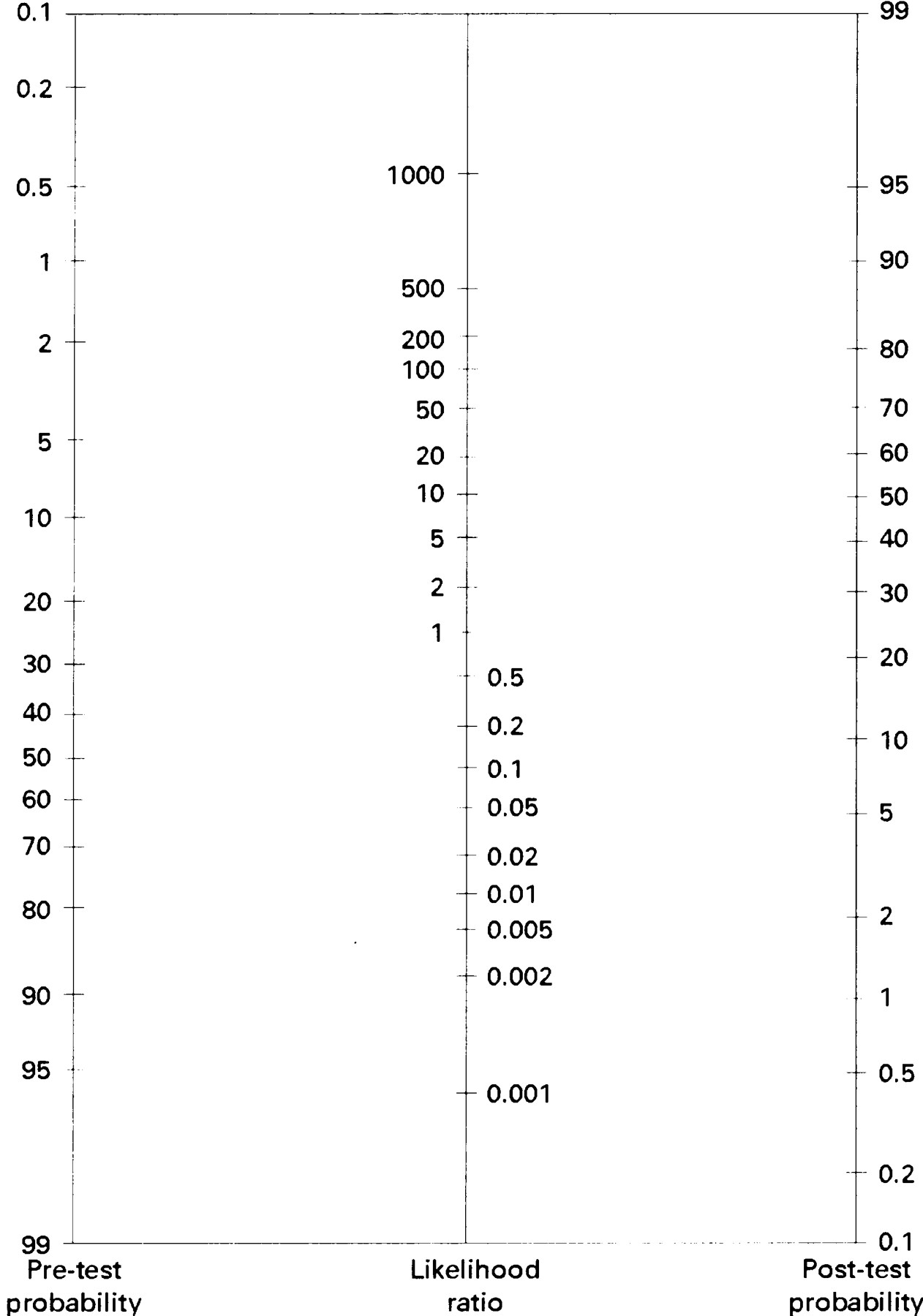
One way of summarising the findings of a study of a diagnostic test for using in a clinical situation where there is a different prevalence is to use the likelihood ratio.The likelihood ratio for a positive test result is the likelihood that a positive test comes from a person with the disorder rather than one without the disorder [A / (A + C)] / [B / (B + D)], or sensitivity / (1 − specificity). In the example this is (32 / 33) / (2 / 103) = 49.94. The likelihood ratio has the advantage that, because it is calculated from the sensitivity and specificity, it remains constant even when the prevalence changes. The likelihood ratio can be multiplied by the pre-test odds, (1 − pre-test probability) / pre-test probability, to produce the post-test odds. Because probabilities are easier to interpret than odds, we usually convert the post-test odds back to the post-test probability, post-test odds/(1 + post-test odds). The post-test probability is the probability that a patient, scoring positive on the diagnostic test, actually has the disorder. Using a nomogram (fig⇓) avoids the need for these calculations: anchor a straight line on the left hand axis of the nomogram at the appropriate pre-test probability and continue the line through the central line at the value of the likelihood ratio (about 50). The approximate post-test probability can then be read directly off the right hand axis—see what the effect is on the post-test probability of varying the pre-test probability while keeping the likelihood ratio constant.

The likelihood ratio for a negative test result can be used in a similar way; it represents the likelihood that a negative test comes from a person with the disorder rather than one without the disorder = [C / (A + C)] / [D / (B + D)], or (1 − sensitivity) / specificity. In the example this is (1 / 33) / (101 / 103) = 0.031.

When there is no diagnostic (gold) standard, raters and tests must be compared with each other to find an indices of agreement. Crude agreement [(A + D) / N] simply counts the number of cases for which 2 raters come to the same conclusion. However, even if the raters did not see the subjects, but made their decision just by tossing a coin, they will agree with each other a portion of the time, just by chance. Kappa (κ) (also referred to as Cohen's κ) corrects for this chance agreement; hence it is also known as agreement beyond chance. Unfortunately, κ is also affected by the base rate. If the prevalence is <20% (or >80%) it is almost impossible for κ to be much above 0.20 or 0.30.

When the new scale and the diagnostic (gold) standard are measured on a continuum, or when 2 raters use a continuous scale, then reliability indices are based on correlational statistics. Until recently, the statistic most often used was the Pearson product moment correlation coefficient, abbreviated as r. However, there is no acceptable way of calculating r when there are more than 2 raters; and r is not sensitive to the situation where 1 rater might be consistently higher than the other. For these reasons, r is more often replaced by the intraclass correlation coefficient (ICC). There are actually many different ICCs which can be used depending on whether each rater evaluates every patient or not; the raters are a random sample of all possible raters; or are the only ones the researcher is interested in, and so on.

• Download figure
• Open in new tab
• Download powerpoint

Figure Nomogram for interpreting diagnostic test results. Figure courtesy of DL Sackett. Reproduced with permission from Fagan TJ. New England Journal of Medicine 1975;293:257.